Model Evaluation
Before deploying a model to be consumed by several applications, we need to know what is the expected performance that it will achieve. After training a model using the collected and transformed dataset, concrete metrics have to be calculated so we can have a vision of how well the algorithm can model the data that we have on hand.
Depending on the type of the problem (supervised, unsupervised, classification, regression), there are different metrics to evaluate. In supervised learning, we have available target values that we can use to compare to what was predicted by the model. However, the metrics are different between classification and regression problems since in the first one the target variable is not continuous.
Another topic worth mentioning, that can lead to misleading conclusions, is what data should be used to evaluate. If we train the model with the entire dataset, make predictions over the same dataset, and compare these predictions with the actual values, we are not verifying how the model behaves with unseen data samples. That's why before speaking about evaluation metrics, we have to jump into data split strategies, to be able to separate the data into different sets depending on their use.
Data Split Strategies
A data split strategy is a way of splitting the data into different subsets, so each subset is used with a different goal. This will prevent us from using the entire dataset for training, tuning , and evaluating which can give false conclusions.
The most used strategies are:
- train-test split
- cross-validation
- leave one out
Train-test split
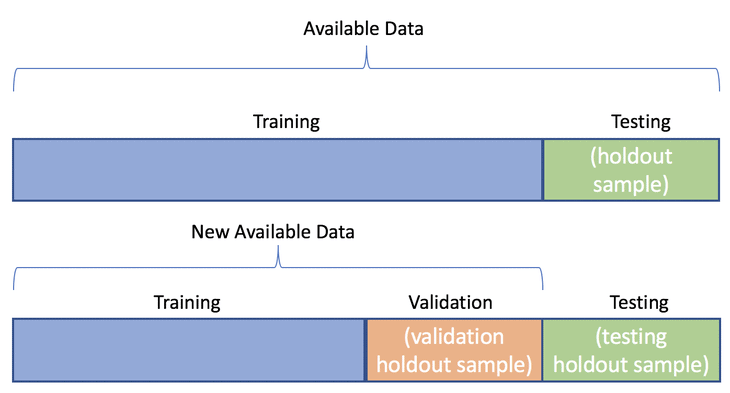
The idea behind the train-test split, as the name suggests, is to split the entire dataset in different sets, usually the following:
- training set (usually ~70%): data samples used to train the model
- validation set (usually ~15%): data samples used to tune the model (hyperparameters, architecture)
- testing set (usually ~15%): data samples used to evaluate the model

Cross-validation
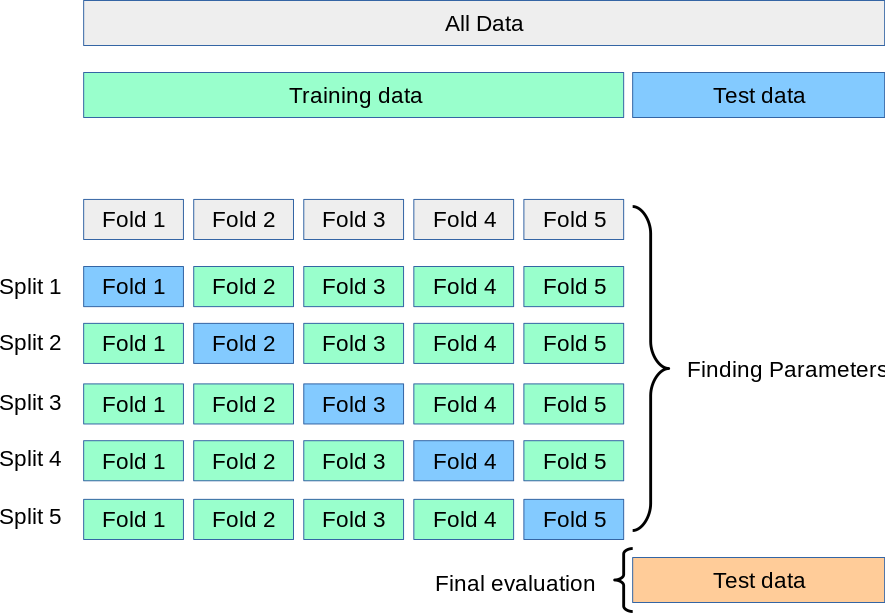
Cross-validation, and leave one out are strategies used usually when the dataset size is not huge, since they are computationally expensive. The idea is to divide the entire dataset into K folds. The model will be trained using N - 1 folds and evaluated on the remaining fold. These will be performed K (number of folds) times, so the advantage is that the data coverage will be higher (more reliable evaluation).

Leave one out
Leave one out is usually applied on small datasets. It is a particular case of cross-validation, it is equivalent to using cross-validation with N folds, given that N is the number of samples in the dataset. This means that the model will be trained and evaluated N times, and the prediction for evaluation will be performed on a single sample at a time.
To be aware
It is worth mentioning two additional topics:
-
temporal data: when dealing with temporal data, it is important to sort before applying the split, because it is considered "cheating" if the sort operation is not applied. Imagine having past and future samples in the training set of a sample in the test set. This would not reflect the real usage of the model;
-
stratification: in classification problems, it is important to maintain the class distribution along the different sets, so we can avoid having, for example, a test set with samples of a single class.
Evaluation Metrics
Evaluation metrics can be divided into regression and classification since the output is different depending on the type of the problem. However, the goal of these metrics is to evaluate how well the model can make predictions. It receives as input the actuals (y) and the predicted values for the same samples (ŷ).
Regression
In regression, the actuals and the predicted values are continuous. The following metrics are usually used to evaluate this kind of models:
- Mean Absolute Error (MAE)
MAE is the easiest metric to interpret. It represents how much the predicted value deviates from the actual value. n is the number of samples (size of y and ŷ).
MAE = (1/n) * Σ|yi - ŷi|
- Mean Square Error (MSE)
MSE is very similar to MAE. The difference is that it is squared instead of using the absolute difference. This will penalize higher errors. It is usually used as a loss function in some of the models (i.e Neural Network).
MSE = (1/n) * Σ(yi - ŷi)²
- Root Mean Square Error (RMSE)
RMSE is the root of MSE. This facilitates the interpretation since it converts the unit from squared to the original unit.
RMSE = sqrt((1/n) * Σ(yi - ŷi)²)
- R-Squared Score (R2)
R2 is a metric that represents how much variance of the data was successfully modeled. It indicates how well the model could represent the data and can establish a relationship between the independent variables and the dependent variable.
SSres is the residual sum of squares, and SStot is the total variance contained in the target output y. This metric is within the range of 0.0 to 1.0, being 1.0 a perfect model, able to represent the entire variance. It can also have negative values in cases where there is a terrible relationship between the target and independent variables.
R2 = 1 - (SSres / SStot)
Useful Plots
Visualization sometimes can help taking conclusions about the obtained results. The listed metrics in the previous section are good to have a clear and specific evaluation of the model. However, some useful plots can be visualized to complement the achieved numeric results.
Regression
The first plot is the actuals vs predicted values. Ideally, all the points should be laid in the diagonal line, which represents that the predicted value is equal to the actual value. This plot gives an overall idea of the achieved predictions and how far they are from the actual value.

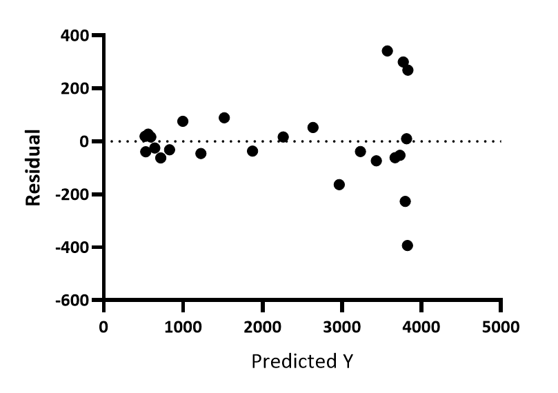
The second one is similar, however, the residual value substitutes one of the previous variables (actuals or predictions). Ideally, the points should be near 0.0 which means no error. The goal of this plot is to conclude the error for each range of values and visualize possible trends that the errors may show. This indicates that there is some pattern contained in the data that the model was not able to cover.

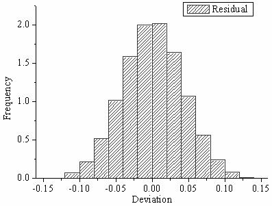
The last one is the histogram of residuals. This allows the conclusion of where are most errors contained. Additionally, it is also important to conclude the distribution of the errors. For example, a Linear Regression assumes that the errors are normally distributed.
